2. Methods: Causal Inference

Comparative Politics

Back to Nogales

We want to test our theory of development: \(X \Rightarrow Y\)

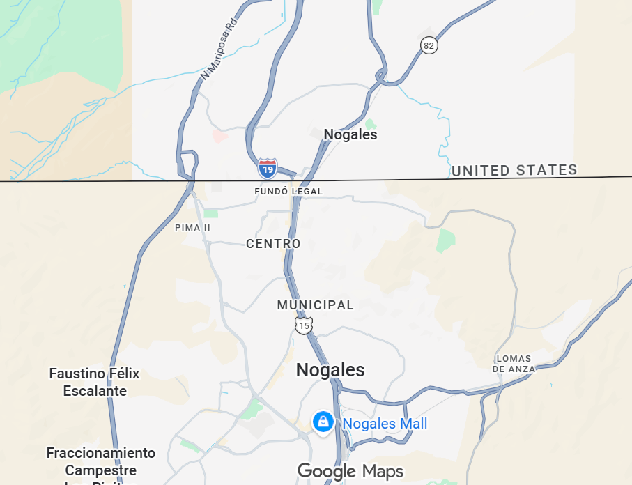
This requires a though experiment: without some factor (\(X\)), N (US) would have been like N (MX)

Central to the though experiment is the counterfactual (what if…)

Testing Theories in Comparative Politics

Comparativists formulate and test theories of politics

• Theories typically contain causal statements: \(X \Rightarrow Y\)
  • “Changing \(X\) causes a change in \(Y\)”
• Test a causal theory \(\rightarrow\) “does the relationship hold in the data?”
• Key issue: when \(X\) changes also \(Z\) changes. Which one caused \(Y\)?
• Without holding \(Z\) constant we cannot know if \(X \Rightarrow Y\)

Causal inference is the main methodology

• Traditionally there were other tools (case study, controlled comparison)
• Today statistical methods are mainstream \(\rightarrow\) control for several \(Z\)

Our Plan for Today

The basics of causal inference

• What is causality
• What is a counterfactual
• What is a causal effect (individual, average)

Estimate causal effects

• Experiments
• Natural experiments
• Common research designs

Basics of Causal Inference

Causal Research Questions

We start by formulating a hypothesis, derived from a theory

Majoritarian electoral systems reduce taxation

This hypothesis is causal. It says that MAJ cause the level of taxation.

It implies two counterfactual states of the world

• Countries with MAJ would have lower tax rate if they did not have MAJ
• Countries without MAJ would have higher tax rate if they had MAJ

Causal Effects

Consider a country under two different counterfactual conditions:

The only difference between the two conditions is the treatment (MAJ or not), everything else is the same

Causal Effects

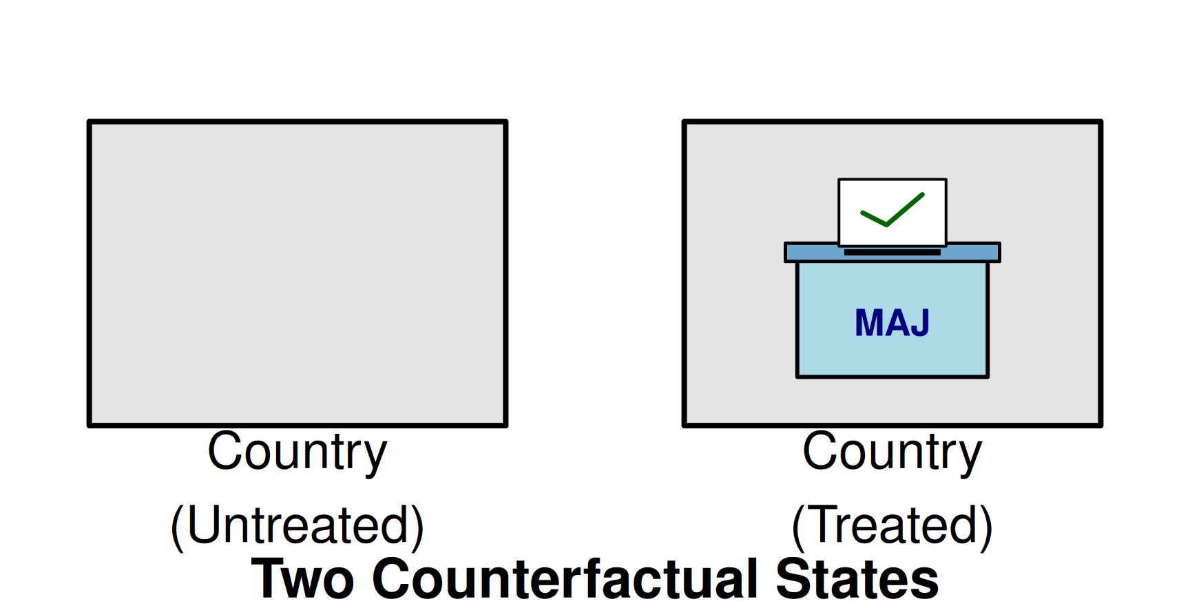
Consider a country under two different counterfactual conditions:

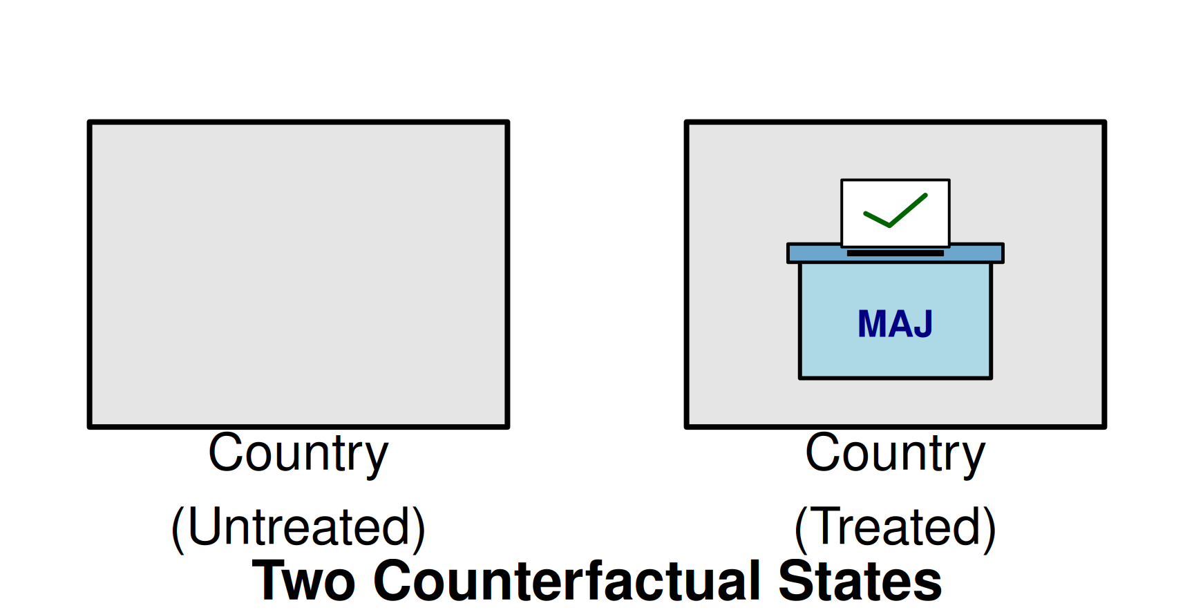
\(Y\) is the outcome variable (e.g., tax rate, tax revenue as % of GDP)

Unit treatment effect (UTE) = difference in country’s \(Y\) between the two conditions

Average treatment effect (ATE) = average of the UTE for all countries

Causality and Counterfactuals

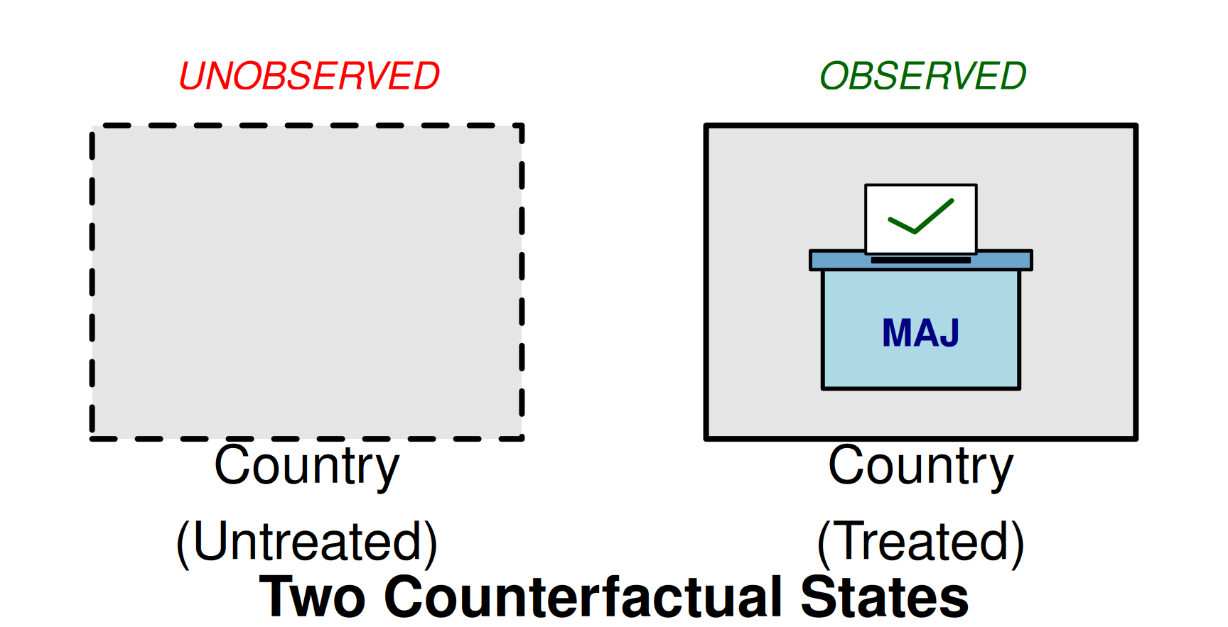
The problem is that a country either has an ES or it has another. It can’t have both together. This is the fundamental problem of causal inference

The Fundamental Problem of Causal Inference

We cannot observe the same unit under two conditions, so the unit treatment effect cannot be observed

Average Treatment Effects

Suppose electoral systems (treatment) are allocated randomly to countries

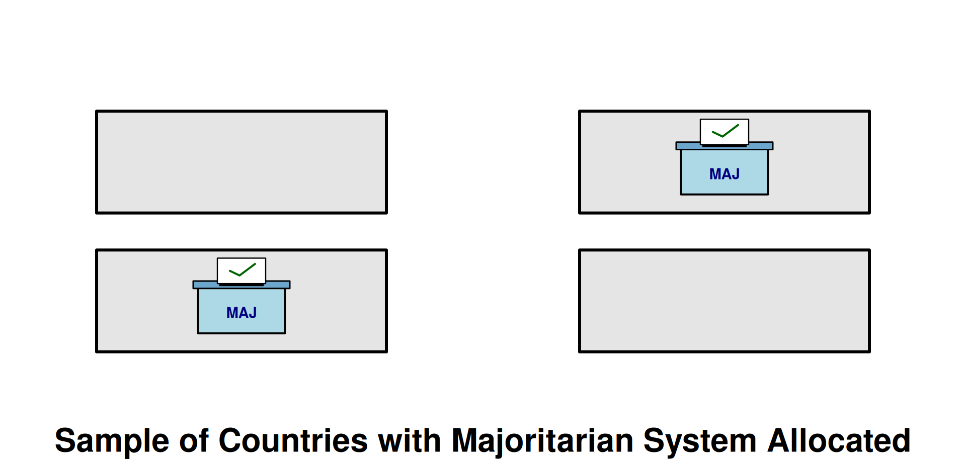
• Countries with MAJ \(\rightarrow\) treatment group
• Countries without MAJ \(\rightarrow\) control group

\(\implies\) Random assignment allows to identify the ATE

The Benefits of Randomization

\(\implies\) Random assignment allows to identify the ATE

Key intuition: random assignment is “blind” to any differences between units. On average, the control group is very similar to the treated group if it were not treated

• Example 1: students’ height
• Example 2: testing drug pill in hospital

\(\implies\) In causal inference, we typically focus on the ATE.

Estimate an Effect Under Random Assignment

If electoral systems were randomized across countries, we could simply compare the average \(Y\) between the treated and control group.

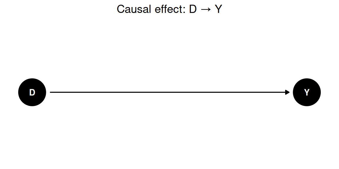
We can do this with a linear regression.

\(Y = \alpha + \beta D + \varepsilon\)

• \(Y\) = taxation outcome (e.g., tax rate)
• \(D\) = variable that indicates whether a country has MAJ (1=yes, 0=no)
• \(\beta\) = estimate of the ATE

When We Can’t Run an Experiment

To estimate the ATE of \(X\) on \(Y\) we need to randomly change \(X\)

• Scientists conduct randomized experiments
• In political science, randomization often unfeasible or unethical
• In these cases, we look at events that have already happened
  • Use observational data and look for natural experiments

We then need identification assumptions about the “randomness”

• E.g., assume the electoral system was somehow chosen by chance
• We can do causal inference only if these assumptions are very plausible
• This depends on our knowledge of the assignment process

The Problem of Endogeneity

Imagine that countries adopt electoral institutions based on economic conditions: richer countries are more likely to adopt MAJ

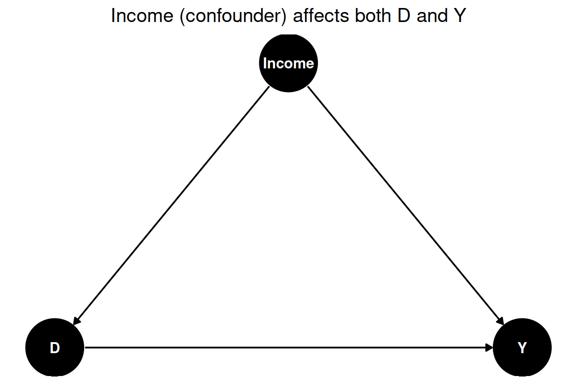
If we simply compare treated and non-treated countries as before, and run \(Y = \alpha + \beta D + \varepsilon\), we will get:

\[\beta= \text{ATE}\] \[+ \underbrace{\text{prior income differences}}_{\text{bias}}\]

We call this selection or endogeneity or confounding or omitted variable.

\(\implies\) “correlation is not causation”

Address Endogeneity

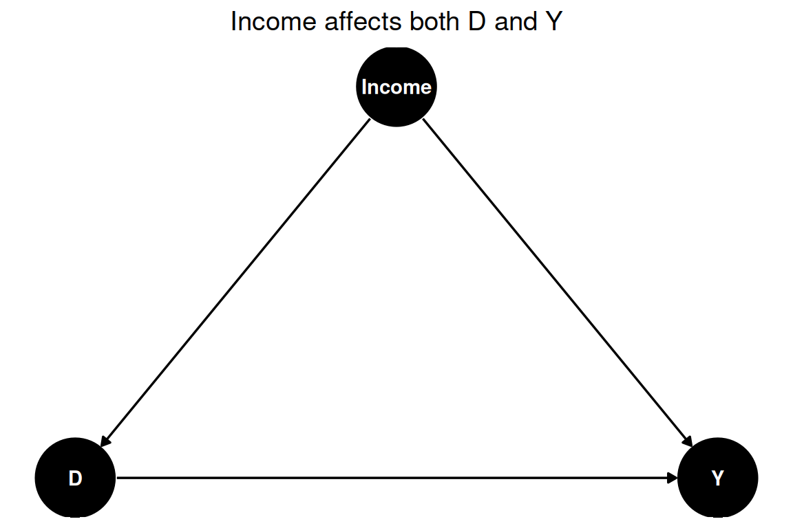
If we include income in a multivariate regression, we “keep it constant” and compare units with the same income

\(Y = \alpha + \beta D + \gamma \text{Income} + \varepsilon\)

and now

\(\beta=\text{ATE}\)

Common Forms of Endogeneity

We Need a Causal Research Design

To recap: we want to test a theory that says \(X \Rightarrow Y\)

• Find a setting where \(X\) can be thought of as random
• Background knowledge on how \(X\) was determined
• If not random, we need to remove the source of endogeneity
• Use statistical methods to estimate ATE

Causal Research Design \(\rightarrow\) select units, comparisons, methods to estimate ATE in a credible way

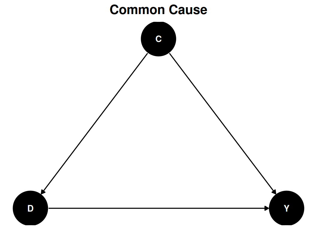
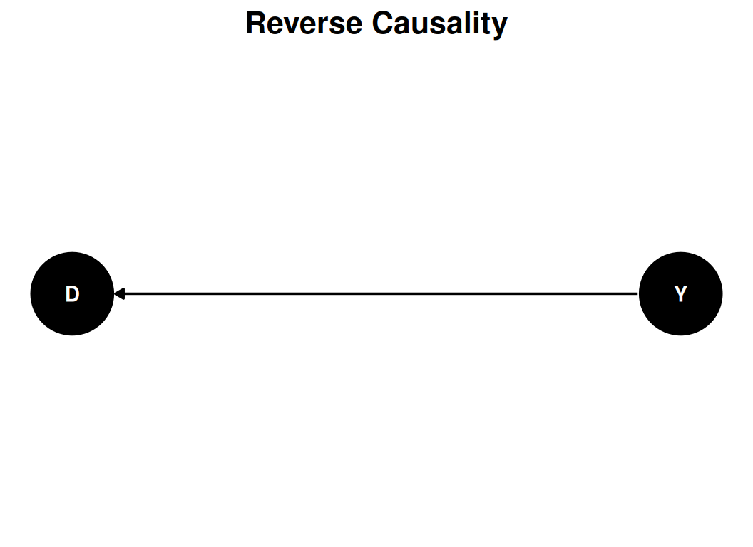
From Between-Country to Within-Country

Common solution: using within-country units reduces endogeneity issues

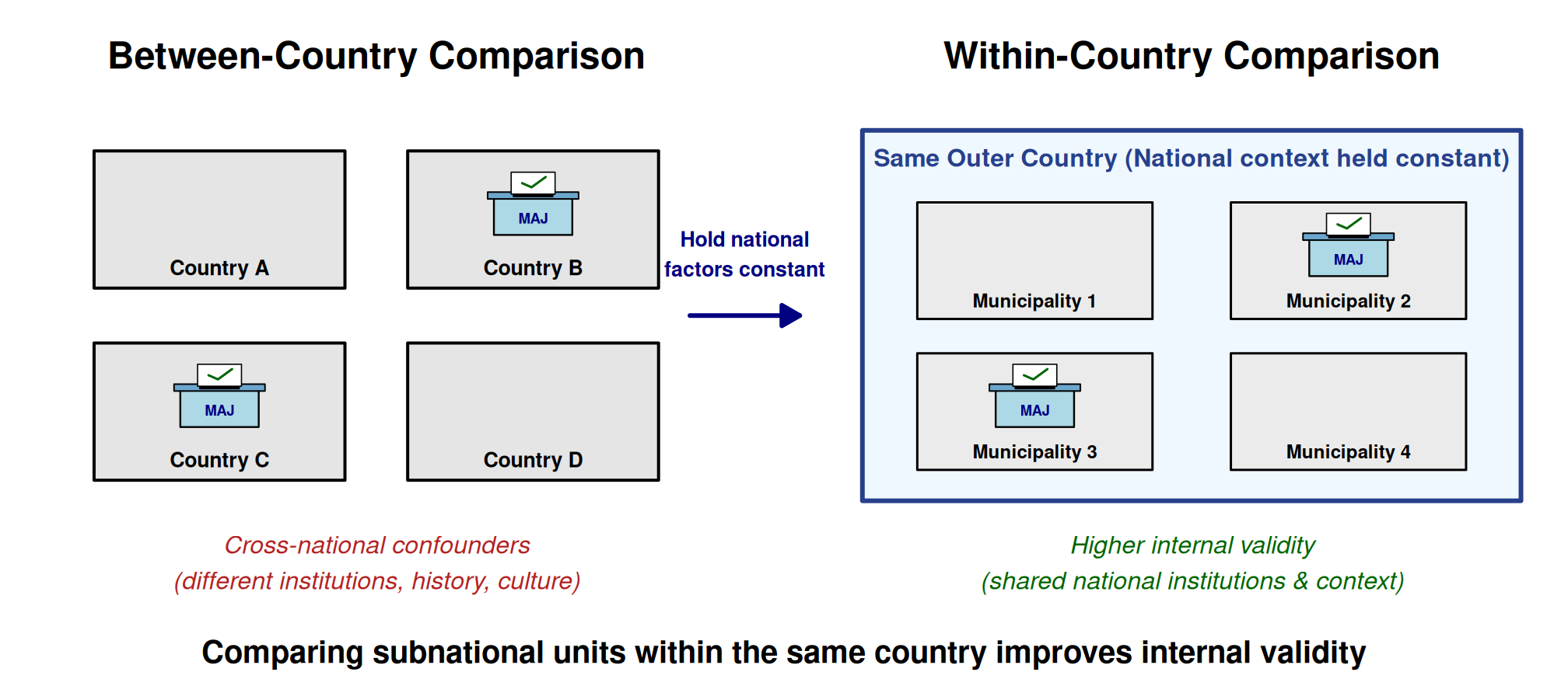
However, this may change the scope of the theory or the relevance

• Civil wars are by definition country-specific
• Within country we can compare specific elements of the same war

Causal Research Designs

Randomized Experiments

The “gold standard” of causal inference

• Field experiments. Treatment administration and outcome measurement in the real world.
  • Widely used in political science and economics
  • E.g., randomize vote encouragement letters to study the effects on turnout
• Survey experiments. Treatment administration and outcome measurement within a survey.
  • Longer tradition in political science to study public opinion
  • E.g., randomize how information is presented to study the effects on voters’ opinion
    
  • Measures psychological mechanisms rather than real-world effects

Control Variables

Endogeneity is due to known variables in the data

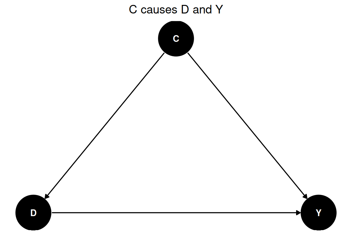
Run multivariate regression that includes the confounder as a control variables

\(Y = \alpha + \beta D + \gamma \text{(control variables)} + \varepsilon\)

Instrumental Variables

Endogeneity is due to unobserved variables (we cannot control), but “part” of the treatment is caused by a random variable

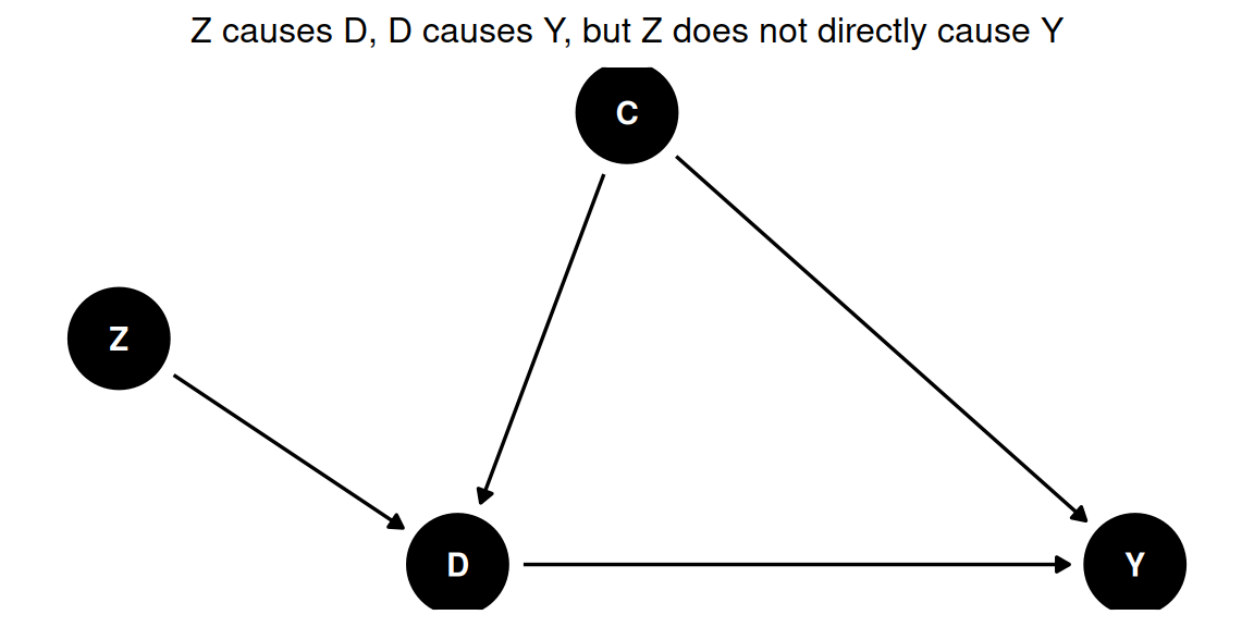
The instrumental variable \(\rightarrow\) exogenous/random and has a causal effect on the treatment (\(\approx\) a random “push” to accept)

Instrumental Variables

Endogeneity is due to unobserved variables (we cannot control), but “part” of the treatment is caused by a random variable

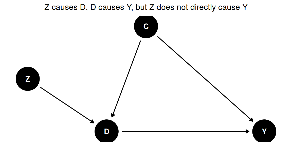
First stage: \(D = \delta + \theta Z + u\)

Second stage: \(Y = \alpha + \beta D + \varepsilon\)

The statistical model estimates the “first stage”, then predicts the values of \(D\) and replaces \(D\) wiht them in the “second stage”

\(\implies\) same as controlling for the “endogenous part” of \(D\)

Difference-in-Differences

Treatment happens in time only for some units

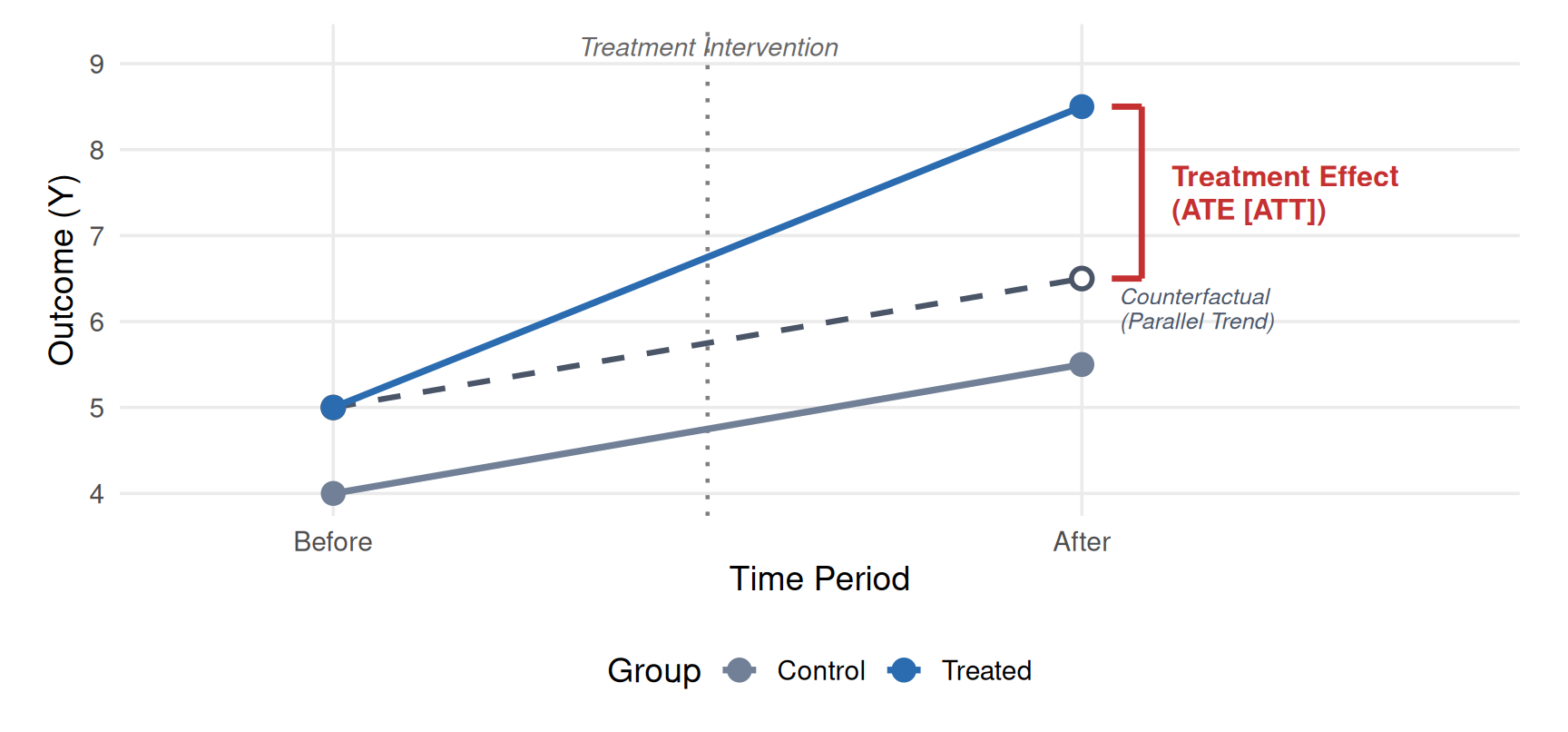
We compare changes between treated units and untreated units

The assumption is parallel trends in absence of treatment

Regression Discontinuity Design

Treatment is applied only/more to units on one side of a cutoff value

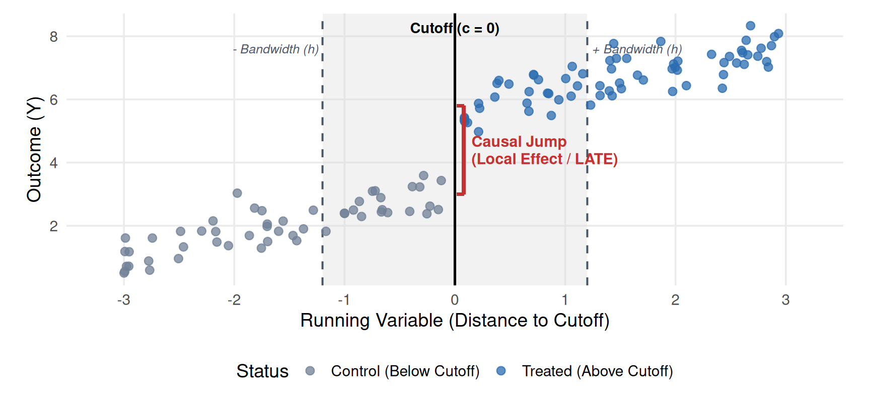
We compare units very close to the cutoff, that are arguably very similar

The assumption is that they cannot alter their score to be on the other side

Summing up

What We Learned Today

• Testing theories means testing causal relationships
• The Fundamental Problem of Causal Inference is the key problem
• Randomization partially solves it \(\rightarrow\) average effects
• Ideally we would always run randomized experiments
• Hardly feasible in political science
• We want to study real-world (observational) data with a causal research design
• We must understand the process of treatment assignment
• Different designs estimate effects under some assumptions

Thank you!